library(sbmr)
library(dplyr)
#>
#> Attaching package: 'dplyr'
#> The following objects are masked from 'package:stats':
#>
#>     filter, lag
#> The following objects are masked from 'package:base':
#>
#>     intersect, setdiff, setequal, union
library(tidyr)
library(ggplot2)
Start with the package included pollinators network.
clements_pollinators %>% head()
#> # A tibble: 6 x 2
#>   pollinator           flower
#>   <chr>                <chr>
#> 1 Acmaeops-longicornis Carduus-hookerianus
#> 2 Acmaeops-longicornis Mertensia-sibirica
#> 3 Acmaeops-longicornis Prunus-demissa
#> 4 Acmaeops-longicornis Rosa-acicularis
#> 5 Acmaeops-longicornis Rubus-deliciosus
#> 6 Acmaeops-pratensis   Prunus-demissa

bind_rows(
  count(clements_pollinators, pollinator) %>%
    transmute(id = pollinator, degree = n, type = "pollinator"),
  count(clements_pollinators, flower) %>%
    transmute(id = flower, degree = n, type = "flower")
) %>%
  ggplot(aes(x = degree)) +
  geom_histogram(binwidth = 1, color = 'white') +
  facet_grid(rows = "type", scales = "free_y") +
  labs(title = "Degree distributions for flower and pollinator nodes",
       subtitle = "Note different y-axis scales")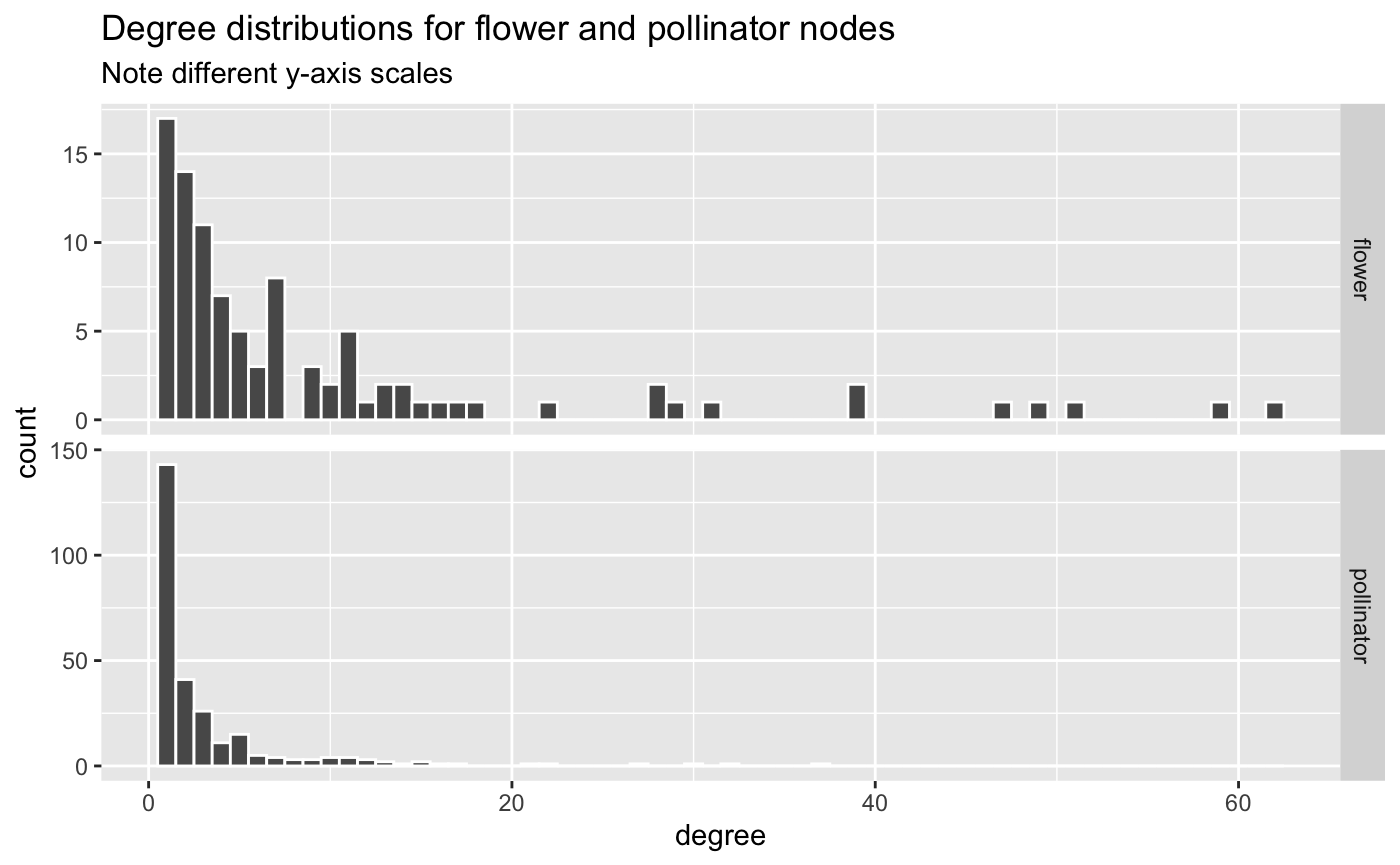
Load into SBM
pollinator_net <- new_sbm_network(edges = clements_pollinators,
                                  bipartite_edges = TRUE,
                                  edges_from_column = pollinator,
                                  edges_to_column = flower,
                                  random_seed = 42)

pollinator_net
#> SBM Network with 371 nodes of 2 types and 923 edges.
#>
#> Nodes: # A tibble: 6 x 2
#>   id                       type
#>   <chr>                    <chr>
#> 1 Achillea-millefolium     flower
#> 2 Acmaeops-longicornis     pollinator
#> 3 Acmaeops-pratensis       pollinator
#> 4 Aconitum-columbianum     flower
#> 5 Agapostemon-coloradensis pollinator
#> 6 Agapostemon-sp.          pollinator
#> ...
#>
#> Edges: # A tibble: 6 x 2
#>   pollinator           flower
#>   <chr>                <chr>
#> 1 Acmaeops-longicornis Carduus-hookerianus
#> 2 Acmaeops-longicornis Mertensia-sibirica
#> 3 Acmaeops-longicornis Prunus-demissa
#> 4 Acmaeops-longicornis Rosa-acicularis
#> 5 Acmaeops-longicornis Rubus-deliciosus
#> 6 Acmaeops-pratensis   Prunus-demissa
#> ...
#>
Visualize it
if(is_html){
  visualize_network(pollinator_net,
                    node_color_col = 'type',
                    node_shape_col = 'none')
}
Run agglomerative merging to find initial MCMC State
pollinator_net <- pollinator_net %>%
  collapse_blocks(desired_n_blocks = 4,
                  num_mcmc_sweeps = 5,
sigma = 1.1)visualize_collapse_results(pollinator_net, heuristic = "delta_ratio")
#> Warning: Removed 2 rows containing missing values (geom_point).
#> Warning: Removed 2 row(s) containing missing values (geom_path).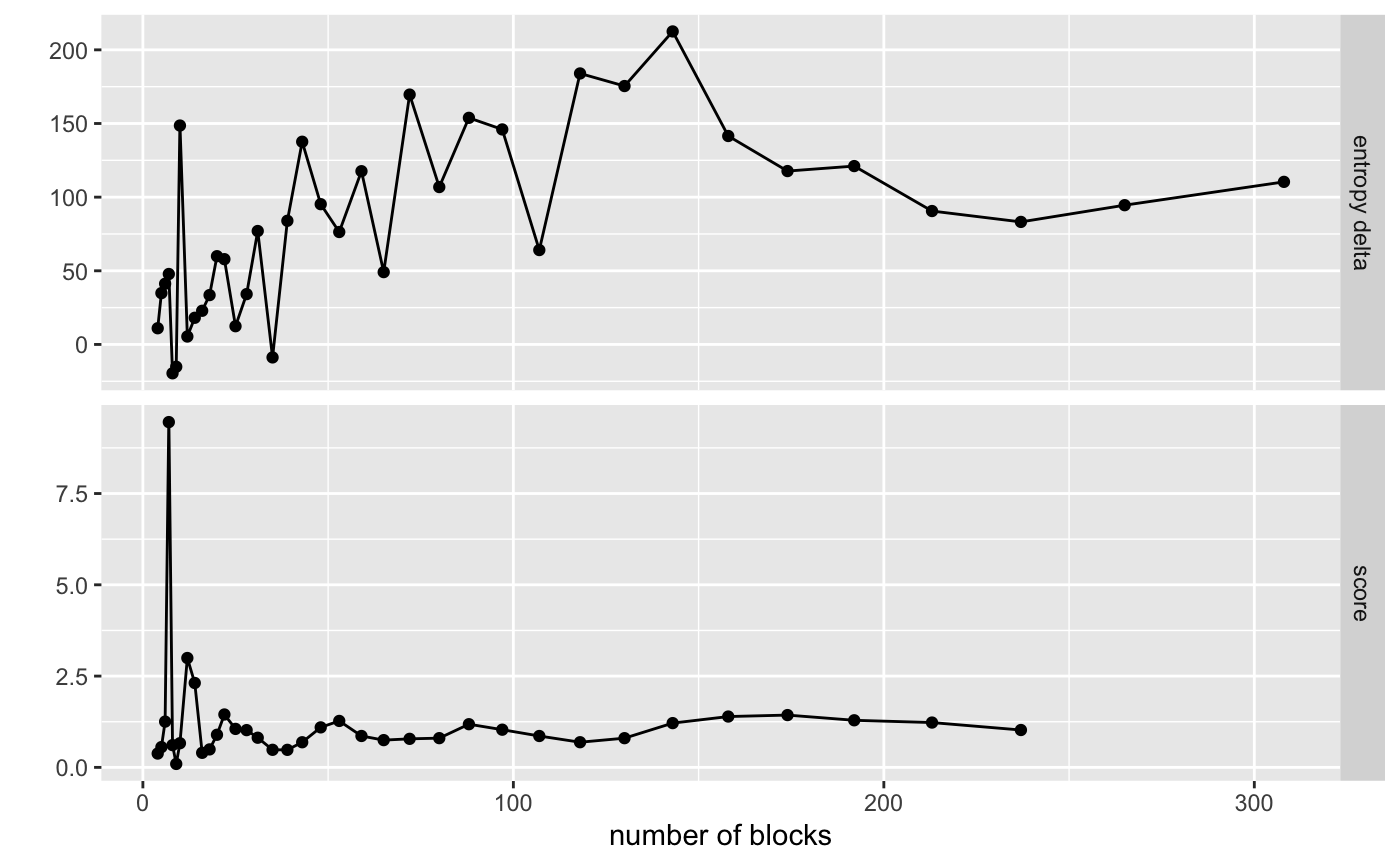 So we have a very clear peak. Let’s select it as our starting position.
pollinator_net <- pollinator_net %>%
  choose_best_collapse_state(heuristic = "delta_ratio", verbose = TRUE)
#> Choosing collapse with 7 blocks and an entropy of 47.8333.
Let’s visualize this result on the network layout
if(is_html){
  pollinator_net %>%
    visualize_network(node_shape_col = 'type',
                      node_color_col = 'block')
}
MCMC Sweeping
We can now run 200 sweeps from the initial position chosen by the collapse…
num_sweeps <- 200

pollinator_net <- pollinator_net %>%
  mcmc_sweep(num_sweeps = num_sweeps,
             eps = 0.1,
             track_pairs = TRUE)

pollinator_net %>%
  visualize_mcmc_trace() +
  labs(title = glue::glue('Result of {num_sweeps} MCMC sweeps'),
       subtitle = "Entropy Delta of sweep and number of nodes moved for sweep")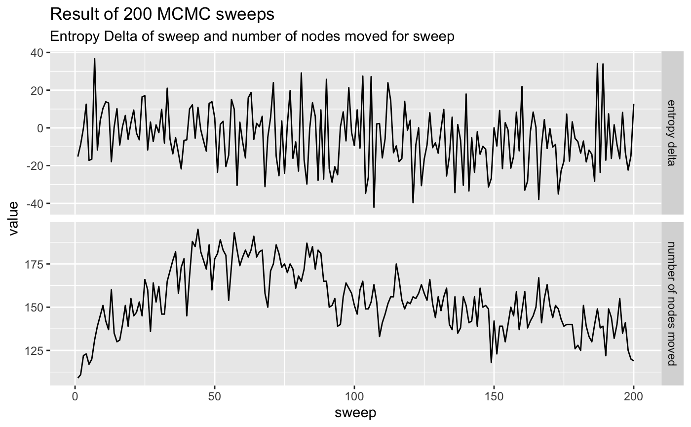
Visualizing propensity matrix
pollinator_net %>%
  get_sweep_pair_counts() %>%
  ggplot(aes(x = node_a, y = node_b, fill = proportion_connected)) +
  geom_raster() +
  theme(
    axis.text = element_blank(),
    axis.ticks = element_blank()
  ) +
  labs(x = "node a",
       y = "node b",
       fill = "Proportion of sweeps\nin same block",
       title = "Node block consensus matrix")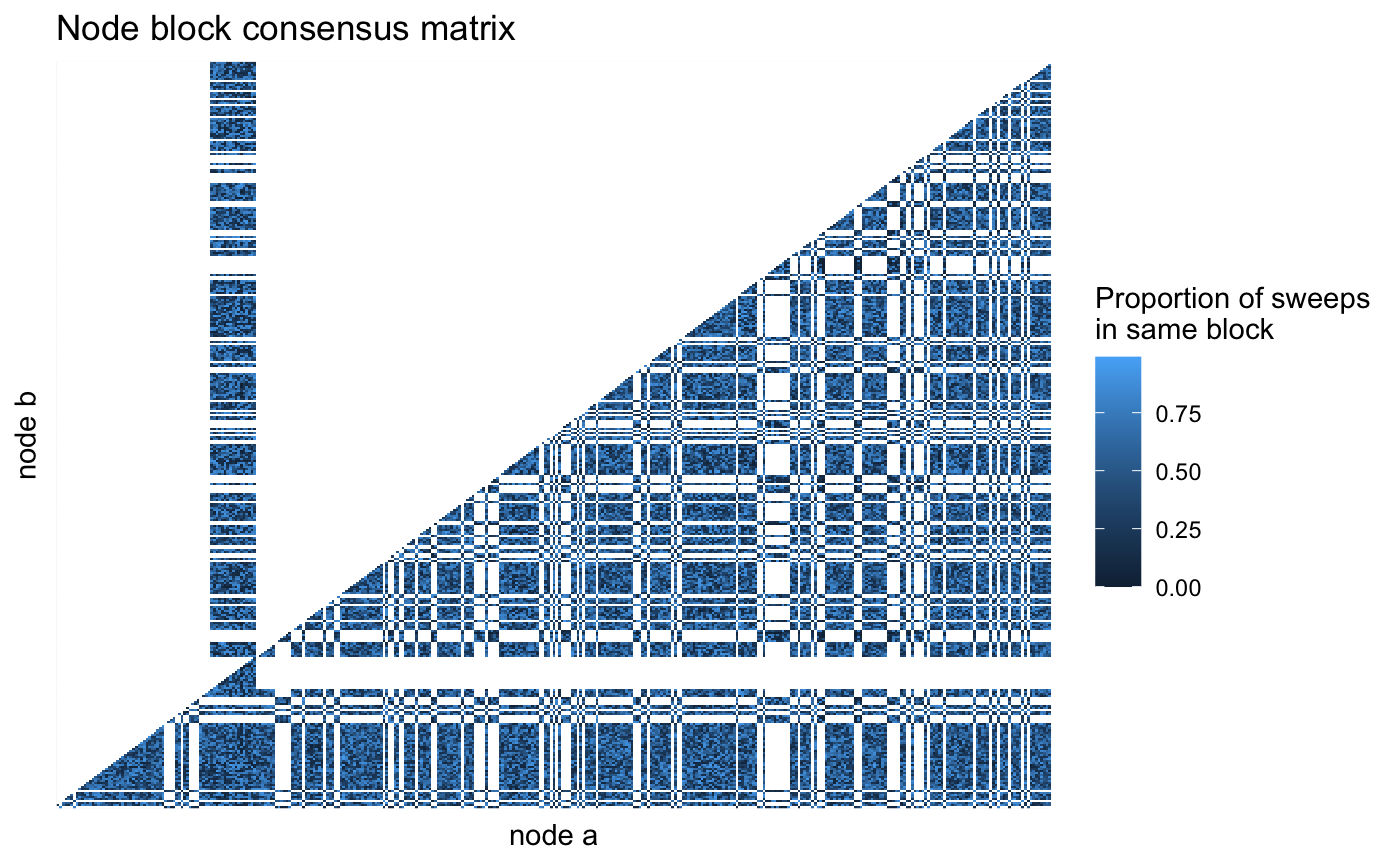
ECDF of propensity distribution
visualize_propensity_dist(pollinator_net)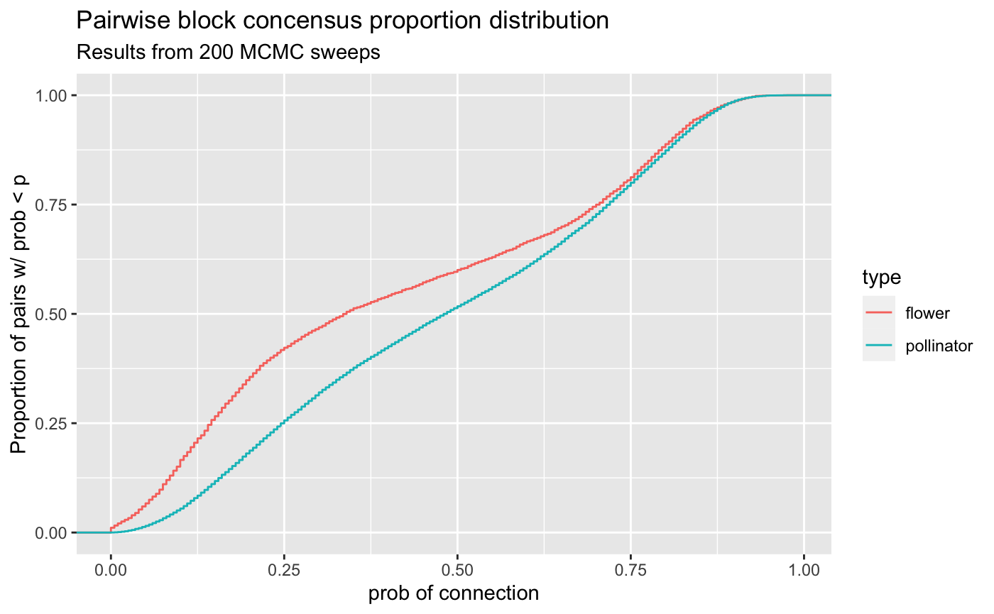
if(is_html){
  pollinator_net %>%
    visualize_propensity_network(proportion_threshold = 0.01,
                                 isolate_type = "flower")
}